After finishing up the Deep Learning Specialization at coursera.org I was very inspired by the power of TensorFlow and the future of deep learning. I wanted to push even further into this exciting area of machine learning and pursue the TensorFlow Developer Certificate.

As part of this learning process I have been spending a lot of time working on computer vision fundamentals. Starting with the “Hello World” of computer vision projects, the famous MNIST handwritten digits dataset, I was able to establish a solid foundation with the TensorFlow basics and continued from there. Using a very simple deep learning model with only a handful of hidden layers I was able to quickly achieve a test accuracy of 98.3% on the multiclass set. A pretty good start!

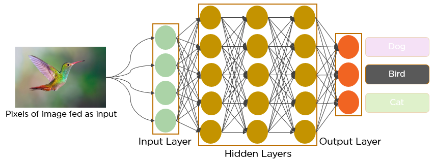
The image below is an example of a simple deep learning network like the one used on the MNIST problem, taking the pixels as input with multiple hidden layers before the softmax output layer predicting the class of the image. Video overview.

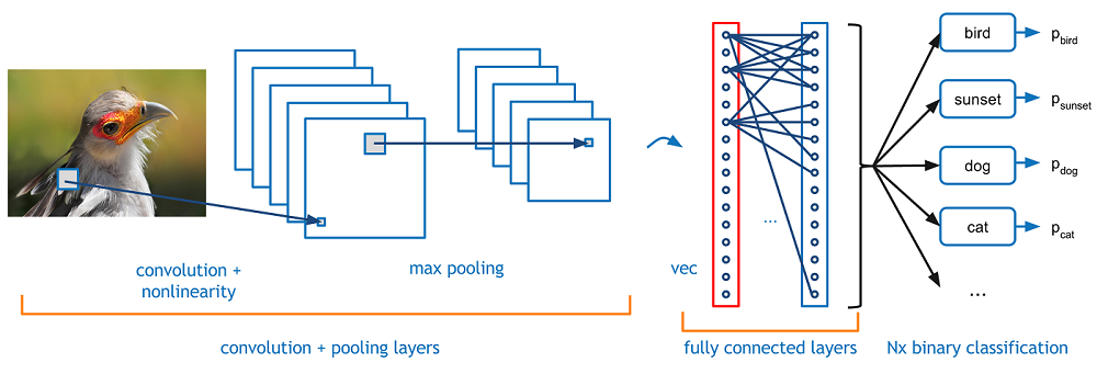
For a more in depth example of the entire computer vision workflow, including data preprocessing and model tuning I chose to work with a much larger and more complex dataset. Another very popular open dataset, CIFAR-10. It is one of the most popular datasets for machine learning research. It contains 60,000, 32×32 colour images in 10 different classes. The classes represent airplanes, cars, birds, cats, deer, dogs, frogs, horses, ships, and trucks. For this problem I used a Convolutional Neural Network. CNN’s are very powerful in computer vision as the convolutional layers are used for advanced feature detection allowing for things like facial recognition software to unlock your phone. These layers act as filters that scan the image for features, a simple example shown below. Video overview.

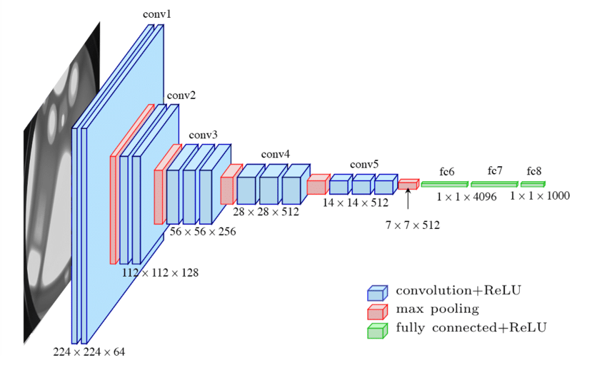
One of the challenges of deep learning is network architecture. Choosing the right architecture for the problem impacts performance and is something that improves with experience. To begin, I chose to mimic the VGG-16 architecture (also called OxfordNet, named after the developers) which is a great building block and easy to implement. The concepts are to include multiple convolutional layers (1-3) in each pooling step. The layers themselves are multiples of 16 (32, 64, 128, etc). An example is shown below.

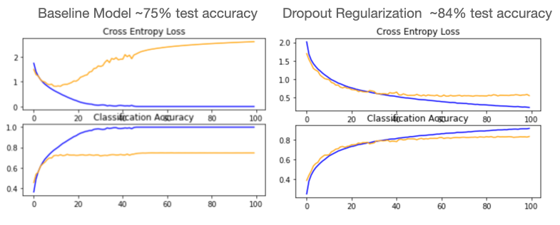
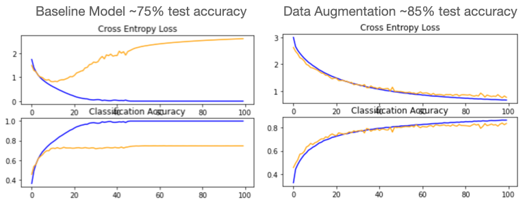
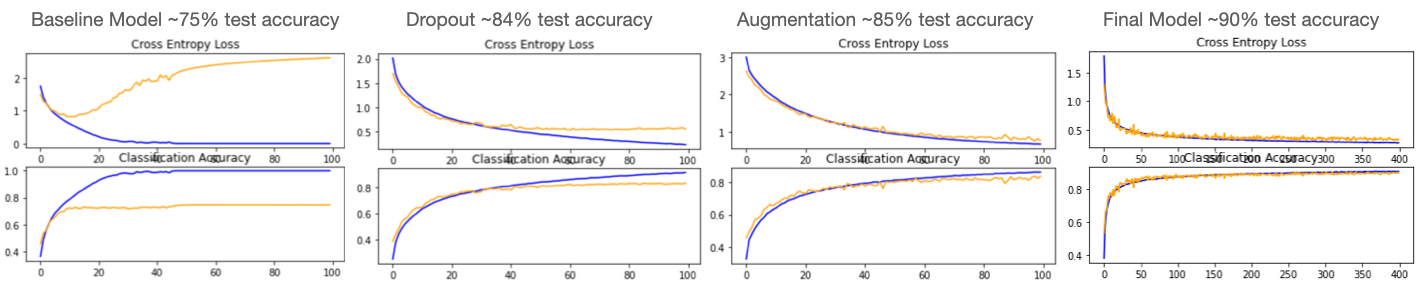
After defining multiple functions to help make the traning and tuning process more efficient by automating preprocessing steps I began building my baseline CNN model. With a basic model an accuracy of ~75% was achieved. That is a pretty good starting point but taking a look at the loss and accuracy curves we can see there is clear room for improvement. The diverging loss curve as well as the obvious overfitting can both be addressed with a technique called Dropout Regularization. This randomly eliminates nodes of a hidden layer to prevent the model from getting “stuck” on certain features. Adding dropout regularization dramatically improved the model, increasing accuracy by 9% and much improved learning curves shown below.

As we can see, however there is still a slight divergence in the curves indicating some further room for improvement. One of the most difficult challenges facing any advanced machine learning problem is a lack of quality training data. With computer vision problems we can implement a technique called Data Augmentation to create a variety of synthetic images similar to the training dataset (rotated slightly, shifted, cropped, zoomed, flipped horizontally or vertically, etc). The great part about this is the augmentation occurs in memory during preprocessing and does not impact the original dataset at all. Utilizing augmentation also significantly improved the baseline model, increasing the accuracy and improving the learning curves as shown below.

There are even more ways to improve this, we can increase the dropout regularization by changing the dropout percentage on each layer as well as train the model longer. Additionally, there is a process called batch normalization to stabilize the learning process which improves performance. Lastly, other optimizers can be used. Stochastic Gradient Descent was chosen initially as it is a more straightforward iterative method. The Adam optimizer has grown in popularity which is an adaptive optimizer (adjusts learning rate) and is capable of handling sparse datasets. Looking at our final model learning curves, the SGD model with dropout regularization, batch normalization, and data augmentation performed very well reaching a test accuracy of 88% however the Adam optimizer won out using the same model achieved a test accuracy of 90%! And we can see the learning curves look very good as well. The entire notebook takes about 6 hours to run on Google Colab with a GPU instance. Improving a model from 75%-90%, not too bad for a days work! Note - the runtime increases dramatically on a CPU, a good example of the impact compute power has had on the deep learning explosion!

This was a great excersize diving deep into the inner workings of computer vision and optimizing a CNN model. If you would like to take a look at the code please check out the GitHub Repo. Looking forward to learning more! This was a great excersize diving deep into the inner workings of computer vision and optimizing a CNN model. If you would like to take a look at the code please check out the GitHub Repo. Looking forward to learning more!